Philosophy based on cross-validation
In chapter 7 of Hastie, Tibshirani, and
Friedman (2009)
the authors emphasize cross-validation estimates the expected prediction
error (or generalization error) of a method. This is in
contrast to estimating such errors for a specific model. There
is a line of work that makes use of cross-validation and inherits its
inferential focus on a method rather than a specific model chosen by
that method (Wasserman and Roeder 2009; Meinshausen, Meier, and
Bühlmann 2009; Meinshausen and Bühlmann 2010; R. D. Shah and Samworth
2013) including the focus of this vignette which was proposed
by R. D. Shah and Bühlmann (2018). This paper
and its R implementation (2021) roughly
attempt to answer the question:
Does this method (typically) result in models with a good fit, or does it fail to capture signal that an alternate method could (typically) detect?
If the first method does fit well, then the residuals from that method should (typically) look like pure noise. On the other hand, if an alternate method can predict the residuals with good accuracy (better than noise) that would be evidence the first method is failing to capture some signal. Hence the name RPtests, based on residual prediction. The exact details depend on several (groups of) decisions:
Probability modeling assumptions (foundational, and we will not question these here).\[ \mathbf{y} = \mathbf{X} \beta + \sigma \epsilon \]
The first method, or null method. We want to know if this method is good enough. We will focus on using the lasso (1996) to select variables in a (potentially high-dimensional) linear model. (The high level idea could be applied using other methods as well but that would require changing some other details in the implementation).
One or more secondary or alternate methods that could be chosen depending on what type of model misspecification we are concerned about. We will focus on whether we should include more predictor variables, but another possibility is to search for non-linear relationships. (An alternate method could be a hybrid or ensemble of several methods, but we will not explore this here).
Analysis/pipeline choices including how to tune each method, estimating the variance of the noise, number of bootstrap samples, and so on. (We will also not question these here).
We’ll focus on one of the main cases investigated in (R. D. Shah and Bühlmann 2018): testing a linear model against an alternative that includes additional predictors. To determine if the alternative predicts the residuals significantly better than noise the paper uses a parametric-residual bootstrap described below, but first we consider an important point about the dimension of the first (null) model.
Low vs high-dimensions
In the low dimensional linear model case, the scaled residuals
\[ \hat{\mathbf{R}} = \frac{(\mathbf{I} - \mathbf{P})\mathbf{y}}{\|(\mathbf{I} - \mathbf{P})\mathbf{y}\|_2} \]
are a pivotal quantity under the null hypothesis that the model fits
(and \(\mathbf P = \mathbf{X}(\mathbf{X}^T
\mathbf{X})^{-1} \mathbf{X}^T\) is the projection or hat matrix).
In this case the distribution of the residuals does not depend on any
unknown parameters, so we can use that distribution for valid hypothesis
tests or other inferences. This is the basis of the standard \(F\)-test for goodness-of-fit, the one
reported at the end of a summary(lm(y ~ x)).
set.seed(1)
x <- runif(50)
y <- x + rnorm(50)
summary(lm(y ~ x))
#>
#> Call:
#> lm(formula = y ~ x)
#>
#> Residuals:
#>     Min      1Q  Median      3Q     Max
#> -1.9115 -0.5747 -0.1463  0.5103  2.2936
#>
#> Coefficients:
#>             Estimate Std. Error t value Pr(>|t|)
#> (Intercept)  0.06272    0.29121   0.215   0.8304
#> x            1.06779    0.48788   2.189   0.0335 *
#> ---
#> Signif. codes:  0 '***' 0.001 '**' 0.01 '*' 0.05 '.' 0.1 ' ' 1
#>
#> Residual standard error: 0.9297 on 48 degrees of freedom
#> Multiple R-squared:  0.09074,    Adjusted R-squared:  0.0718
#> F-statistic:  4.79 on 1 and 48 DF,  p-value: 0.03352
However, this does not work in the high-dimensional case, so (2018) use a combination of previous lasso theory and new technical results to prove the residuals from lasso can be used in a similar way (with slight modifications) to construct tests. The theory relies on fairly standard but strong conditions sufficient for the lasso to estimate the support and signs of the true \(\beta\) with high probability, but (as is typical in lasso theory literature) simulations show good empirical performance under more general settings where the strong sufficient conditions are relaxed.
We briefly note that Janková et al. (2020) apply the same basic idea of predicting residuals to high-dimensional generalized linear models by using the Pearson residuals
\[ \hat R_i = \frac{Y_i - \mu(x_i^T \hat \beta)}{\sqrt{V(x_i^T \hat \beta)}} \]
instead, where \(\mu\) and \(V\) are the conditional mean and variance functions, respectively. However, beyond the basic idea there is much additional work involved in this other case so we do not consider it more here.
Lasso details
To calibrate the test, we need a distribution to compare the accuracy measure (typically) achieved by a null model. In the high-dimensional case the null model is assumed to be selected by lasso with cross-validation. The authors propose iterating the whole procedure multiple times to average over the randomness induced by cross-validation itself. Note that this makes more sense when our inferential focus is the method and not a specific model chosen by the method. Below is a restatement of Algorithm 1 in (2018), the parametric-residual bootstrap procedure for estimating a null distribution. For \(b = 1, \ldots, B\):
- Replace \(\mathbf{y}\) with \(\mathbf{\hat y}\) from the original null
model plus simulated residuals \(\mathbf{\zeta}^{(b)} \sim N(0, \mathbf{I}_{n
\times n})\). (Simulating a new response from the null
model).
- Fit sqrt-lasso (2011) using the above simulated \(\mathbf{y}^{(b)}\) and subtract new fit
\(\mathbf{\hat y}^{(b)}\). (Simulating
residuals achieved by alternative method).
- Normalize simulated residuals and compute some accuracy measure,
such as RSS. (Obtain bootstrap distribution for testing).
Note that the sqrt-lasso method can be replaced with other fitting procedures if we are interested in different alternatives, for example by using a tree based method if we are interested in predictive interactions.
Exercise: why not just predict normalized residuals \((\mathbf{y} - \mathbf{\hat y})/\hat \sigma\) and compare to accuracy in predicting \(\mathbf{\zeta}^{(b)}\)? (Consider dimensions).
RPtest code explanation
Below we do not consider special cases, for example when a
user-specified noise_matrix or beta_est
overrides default behavior. We assume the function is called as
RPtest(x, y, resid_type, test = "group", x_alt) with no
other options changed.
Note: with test = "group" the
RPfunction will be set to lasso_test
regardless of the dimension of the null or alternative.
RPtest
When resid_type = "Lasso" (the default unless otherwise
specified) the following functions will be called.
First, cv.glmnet is run several times (in parallel) to
get an estimate beta_est. The estimated signal is
sig_est <- x %*% beta_est.
Next, comp_sigma_est is called with this
beta_est to compute sqrt(MSE). This is the
noise level used by rnorm, the default
rand_gen, to generate noise terms for simulating
residuals.
Now simulated residuals resid_sim are computed by
calling resid_gen_lasso with the above estimates and noise
terms.
resid_gen_lasso
In parallel, calls resid_lasso which fits square-root
lasso and returns residuals. In the implementation of
sqrt_lasso, if x is not high-dimensional then
you will see warnings saying
Smallest lambda chosen by sqrt_lasso.
If the type is "OLS" then instead of
sqrt_lasso residuals are computed the ordinary way.
Orthogonalizing x_alt
Based on resid_type, this part either uses
sqrt_lasso or OLS to residualize x_alt,
subtracting away predictions based on fits to x_null. By
default x_null = x, the input to RPtest.
Note: At this point, if the input x_alt
is a subset of x, i.e. using the common nested model
structure of \(F\)-tests, this
residualization will practically project x_alt <- 0 in
the "OLS" case or close to it in the "Lasso"
case.
The default RPfunction is lasso_test (when
test = "group")
This is applied on both the original and simulated residuals using
the above orthogonalized x_alt, and will use
glmnet(x_alt, resid[_sim]). As a test statistic it computes
the average MSE over the full solution path using the same values of
lambda as fit to the original residuals.
Summary
After projecting x_alt (approximately, in the Lasso
case) orthogonal to x, it is used with glmnet
to predict the original residuals resid and simulated ones
resid_sim, and the MSE over the solution paths are
compared. If this x_alt predicts the original residuals
better than those simulated from the null then it’s evidence there is
signal in x_alt. To use this as a goodness-of-fit test we
therefore make x_alt include some additional variables
which were not selected in the original fit.
Strategy for goodness-of-fit test
The original model selection algorithm chooses some number of
variables, let’s call this s0. To test for the presence of
signal variables that were not included in this original fit, we choose
a larger sparsity level m * s0 + b with
m >= 1 and b > 0. We use the model
selection algorithm to include more variables up to this level of
sparsity, and we test the significance of these new additional variables
as a way of checking the fit of the original, smaller model.
Simulations and examples
library(RPtests)
library(hdi) # riboflavin dataset
#> Loading required package: scalreg
#> Loading required package: lars
#> Loaded lars 1.3
library(purrr)
library(tidyverse)
#> ── Attaching packages ─────────────────────────────────────── tidyverse 1.3.1 ──
#> ✔ ggplot2 3.3.6     ✔ dplyr   1.0.9
#> ✔ tibble  3.1.8     ✔ stringr 1.4.1
#> ✔ tidyr   1.2.0     ✔ forcats 0.5.1
#> ✔ readr   2.1.2
#> ── Conflicts ────────────────────────────────────────── tidyverse_conflicts() ──
#> ✖ dplyr::filter() masks stats::filter()
#> ✖ dplyr::lag()    masks stats::lag()
devtools::load_all() # this shouldn't be necessary?
#> ℹ Loading unbiasedgoodness
library(unbiasedgoodness)
We continue focusing on the high-dimensional linear model and as an alternative to a selected model we consider whether more variables should be included. Since (2018) are not trying to do selective inference in their simulations it seems there is no model selection involved in choosing the hypotheses. Type 1 error control is shown in simulations set up for the null to be true in all instances, rather than doing model selection and subsetting to instances where the null holds (as in selective inference). In contrast to their simulations, we are interested in the selective (conditional) error control rates, as we explore in the simulations below.
One data generation example
set.seed(1)
n <- 100
p <- 200
s0 <- 5
sim_data <- rXb(n, p, s0, xtype = "equi.corr")
x <- sim_data$x
beta <- sim_data$beta
y <- x %*% beta + rnorm(n)
# True support
which(beta != 0)
#> [1] 1 2 3 4 5
gof_RPtest(x, y)
#> Warning in gof_RPtest(x, y): Sparsity of 1 chosen by cv.glmnet, forcing to 2 for RPtest compatibility
#> $selected_support
#> [1]   5 139
#>
#> $alt_support
#> [1]   3   4  85 133 166 190
#>
#> $pval_full
#> [1] 0.02
#>
#> $pval_full_lasso
#> [1] 0.04
#>
#> $pval_lasso
#> [1] 0.02
#>
#> $pval_OLS
#> [1] 0.02
#>
#> $pval_OLS_beta
#> [1] 0.02
#>
#> $pval_lasso_rev
#> [1] 0.82
#>
#> $pval_OLS_rev
#> [1] 1
Iterate many times
#devtools::load_all()
#library(unbiasedgoodness)
set.seed(1)
n <- 100
p <- 200
s0 <- 5
m <- 1.2
b <- 10

simulate_gof_instance(m, b, n, p, s0)
#>    max_corr   min_beta s_null s_alt null_intersection alt_intersection  null
#> 1 0.5636253 0.03821633      4     6                 4                4 FALSE
#>     alt pval_lasso pval_OLS pval_lasso_rev pval_OLS_rev pval_full
#> 1 FALSE       0.02     0.04           0.24          0.7      0.52
#>   pval_full_lasso pval_OLS_beta
#> 1            0.56          0.06
#devtools::load_all()
#library(unbiasedgoodness)
set.seed(1)
niters <- 1000
sim_results_file <- "./data/glmnet_RPtest.csv"

if (file.exists(sim_results_file)) {
  output <- read.csv(sim_results_file)
  print(paste0(
    "Loading saved simulation results with ",
    nrow(output), " iterates"))
} else {
  # run simulation
  output <- simulate_gof(niters, m, b, n, p, s0)
  write.csv(output, sim_results_file)
}
#> [1] "Loading saved simulation results with 1000 iterates"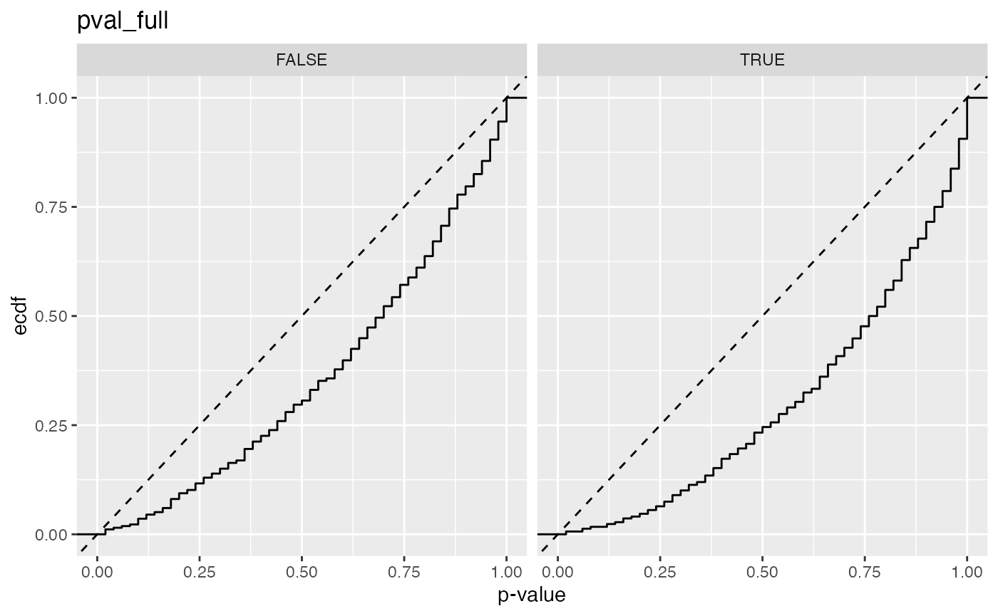
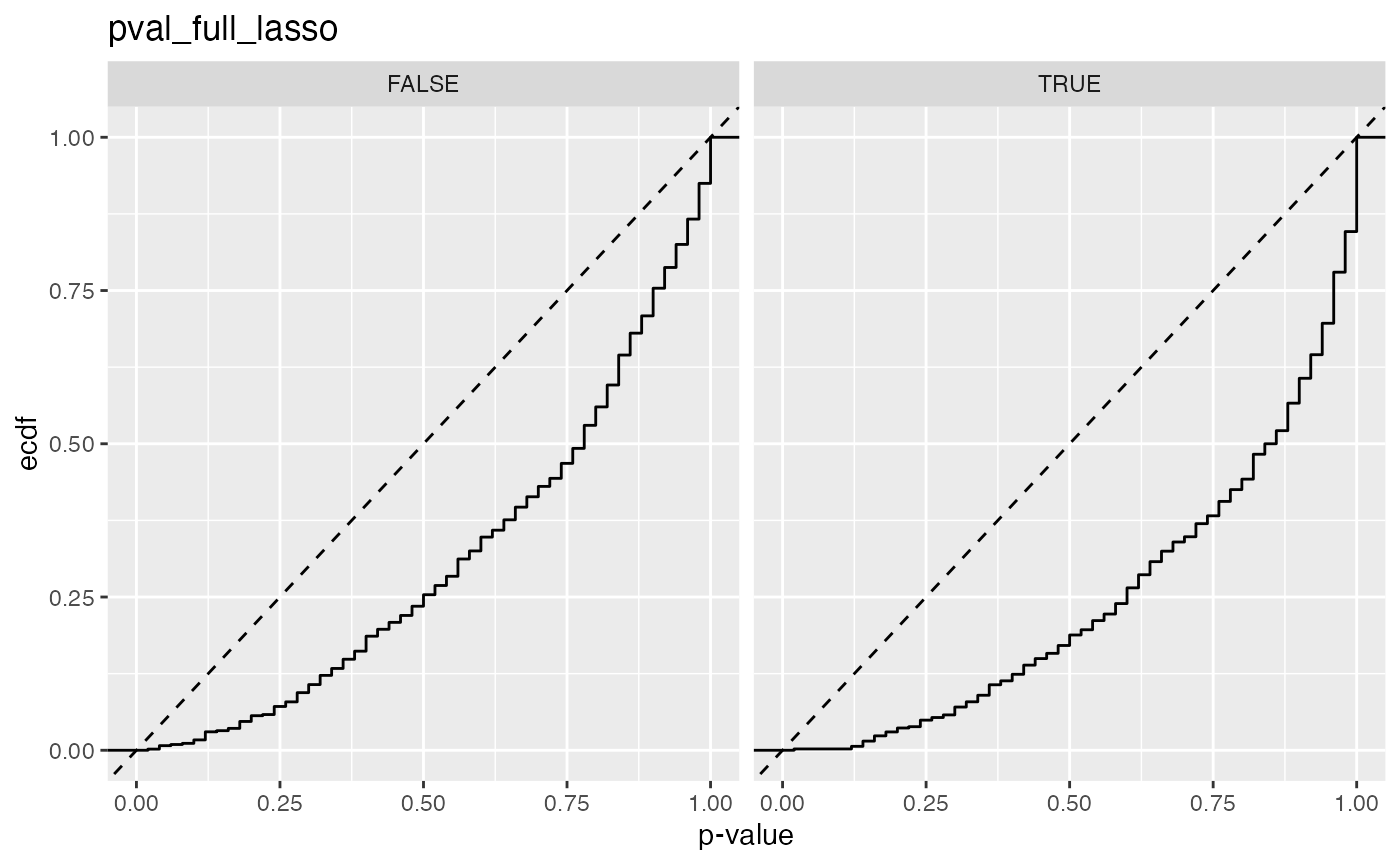
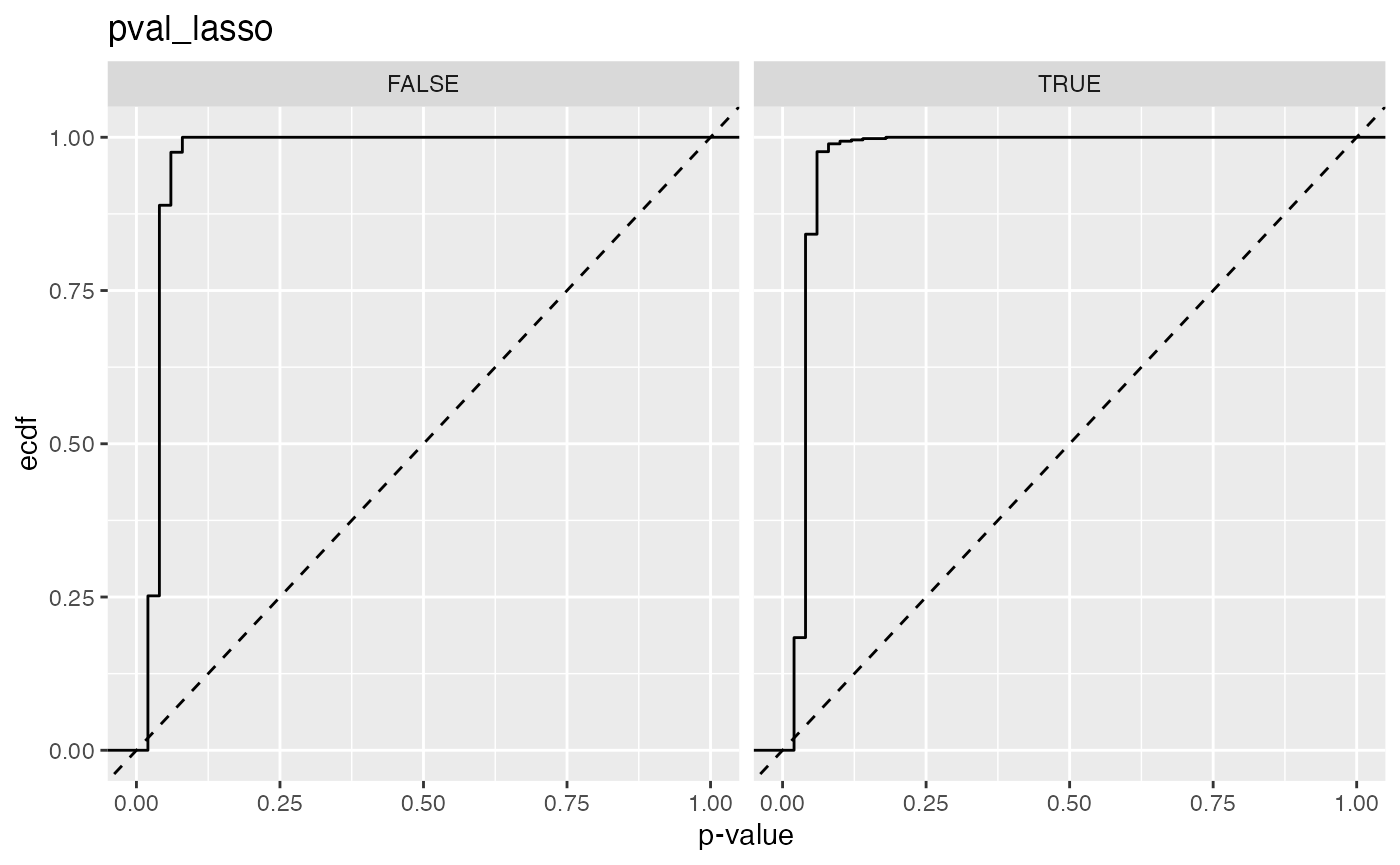
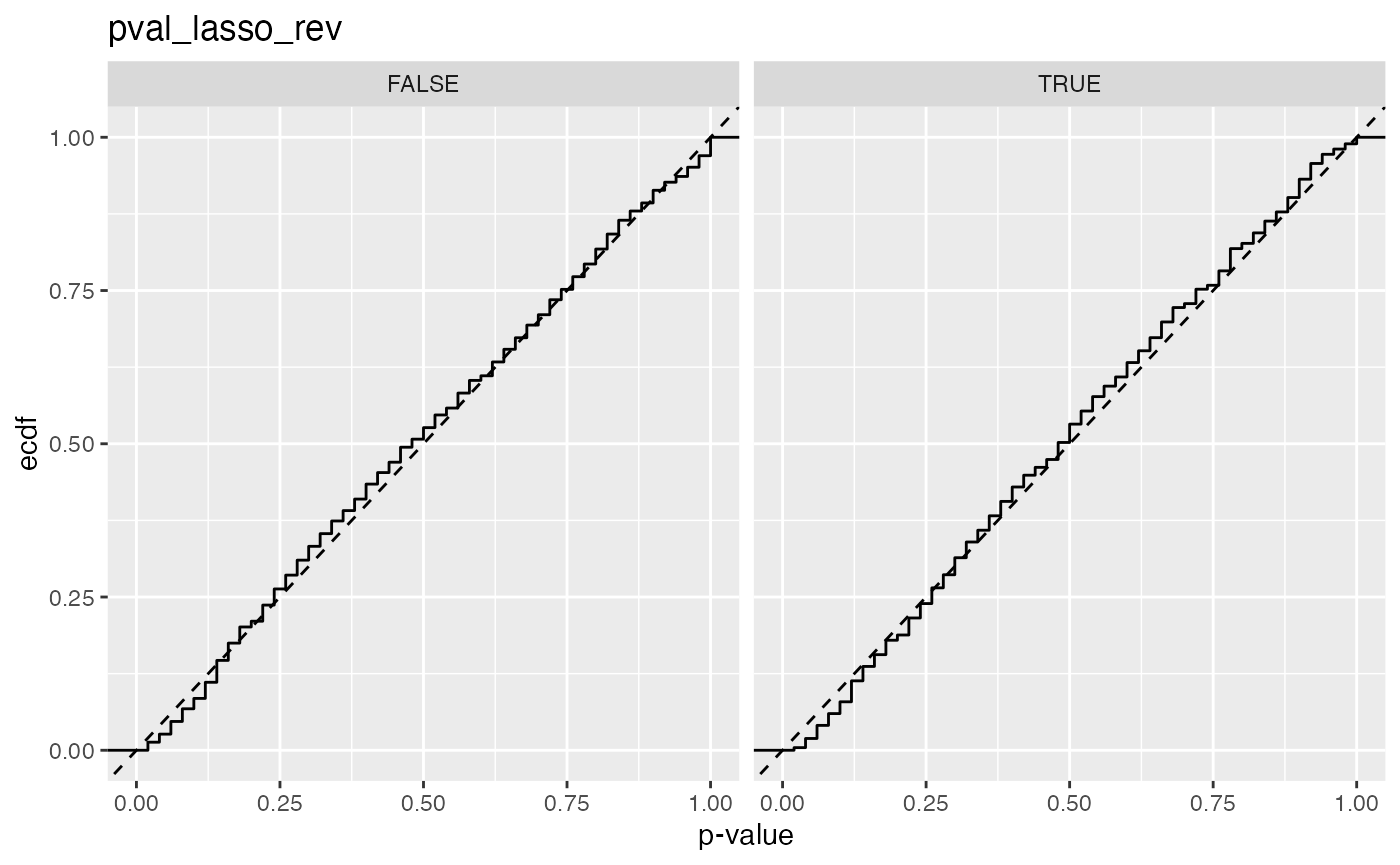

Selective type 1 error rate
output |>
pivot_longer(
starts_with("pval"),
names_to = "type") |>
group_by(type, null) |>
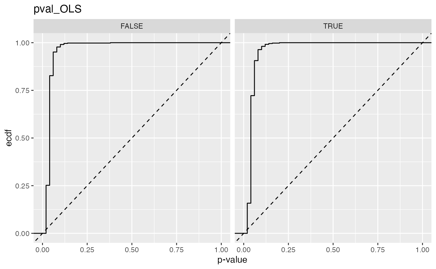
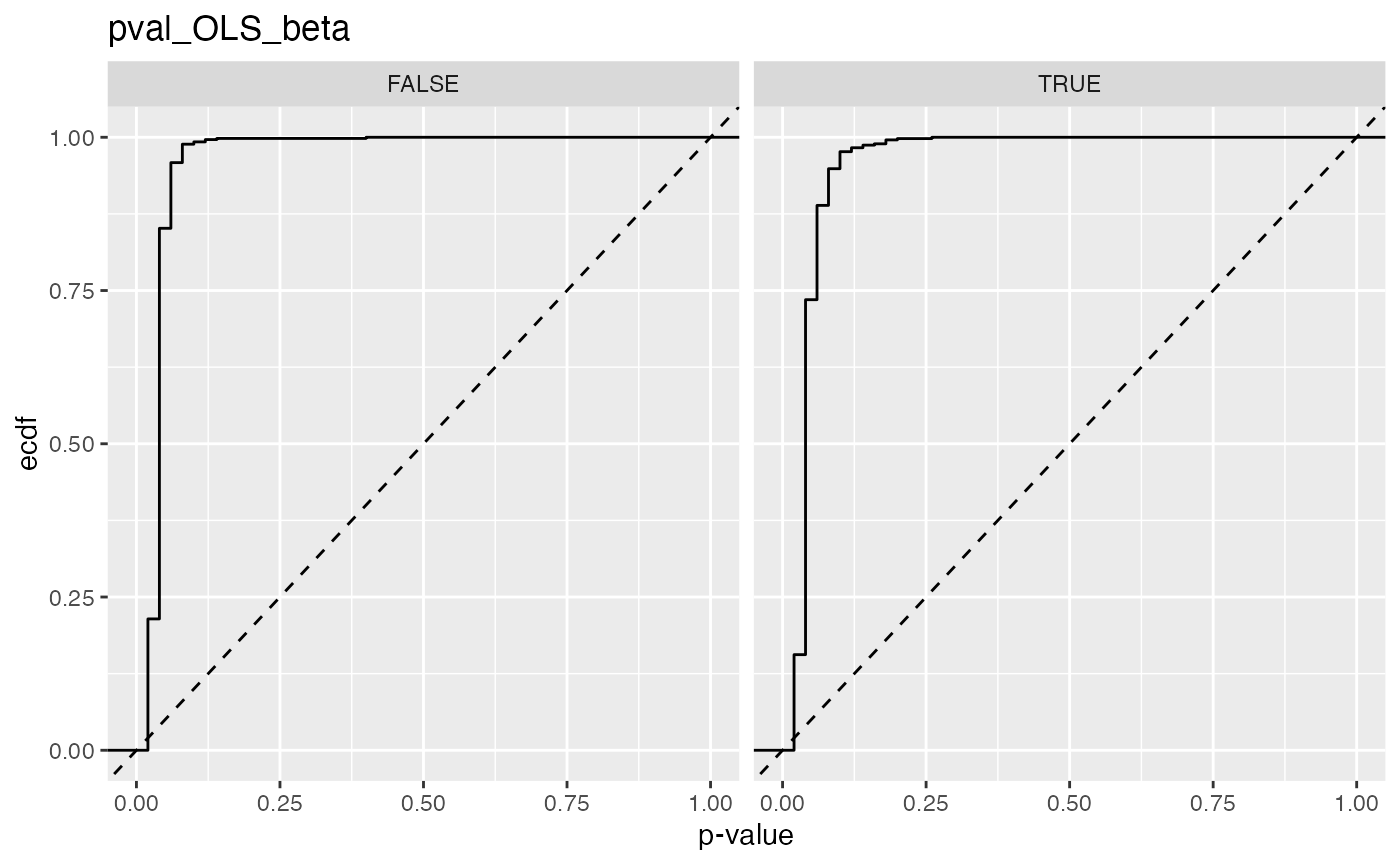
summarize(error_rate = mean(value < 0.05), .groups = "keep")
#> # A tibble: 14 × 3
#> # Groups: type, null [14]
#> type null error_rate
#> <chr> <lgl> <dbl>
#> 1 pval_full FALSE 0.0150
#> 2 pval_full TRUE 0.00641
#> 3 pval_full_lasso FALSE 0.00752
#> 4 pval_full_lasso TRUE 0.00214
#> 5 pval_lasso FALSE 0.889
#> 6 pval_lasso TRUE 0.842
#> 7 pval_lasso_rev FALSE 0.0263
#> 8 pval_lasso_rev TRUE 0.0192
#> 9 pval_OLS FALSE 0.827
#> 10 pval_OLS TRUE 0.722
#> 11 pval_OLS_beta FALSE 0.852
#> 12 pval_OLS_beta TRUE 0.735
#> 13 pval_OLS_rev FALSE 0.0526
#> 14 pval_OLS_rev TRUE 0.0342
output |>
  dplyr::filter(null == TRUE) |>
  pivot_longer(
    starts_with("pval"),
    names_to = "type") |>
  group_by(type) |>
  summarize(error_rate = mean(value < 0.05), .groups = "keep")
#> # A tibble: 7 × 2
#> # Groups:   type [7]
#>   type            error_rate
#>   <chr>                <dbl>
#> 1 pval_full          0.00641
#> 2 pval_full_lasso    0.00214
#> 3 pval_lasso         0.842
#> 4 pval_lasso_rev     0.0192
#> 5 pval_OLS           0.722
#> 6 pval_OLS_beta      0.735
#> 7 pval_OLS_rev       0.0342
Selective power
output |>
  dplyr::filter(null == FALSE) |>
  pivot_longer(
    starts_with("pval"),
    names_to = "type") |>
  group_by(type) |>
  summarize(power = mean(value < 0.05), .groups = "keep")
#> # A tibble: 7 × 2
#> # Groups:   type [7]
#>   type              power
#>   <chr>             <dbl>
#> 1 pval_full       0.0150
#> 2 pval_full_lasso 0.00752
#> 3 pval_lasso      0.889
#> 4 pval_lasso_rev  0.0263
#> 5 pval_OLS        0.827
#> 6 pval_OLS_beta   0.852
#> 7 pval_OLS_rev    0.0526
Model selection success rates
These diagnostics are computed to give some indication of the difficulty level of lasso model selection for the chosen data generation process.
output |>
  summarize(null = mean(null),
            alt = mean(alt),
            s_null = mean(s_null),
            s_alt = mean(s_alt))
#>    null   alt s_null s_alt
#> 1 0.468 0.549  8.583 7.718
output %>% pull(null_intersection) %>% qplot()
#> `stat_bin()` using `bins = 30`. Pick better value with `binwidth`.
output %>% pull(alt_intersection) %>% qplot()
#> `stat_bin()` using `bins = 30`. Pick better value with `binwidth`.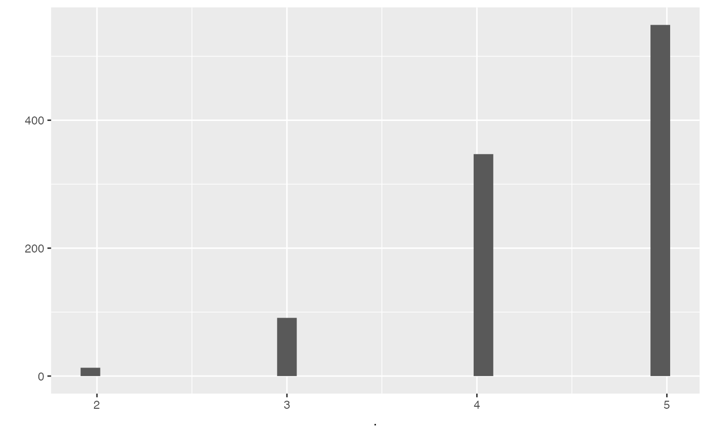
output |> pull(s_alt) |> qplot()
#> `stat_bin()` using `bins = 30`. Pick better value with `binwidth`.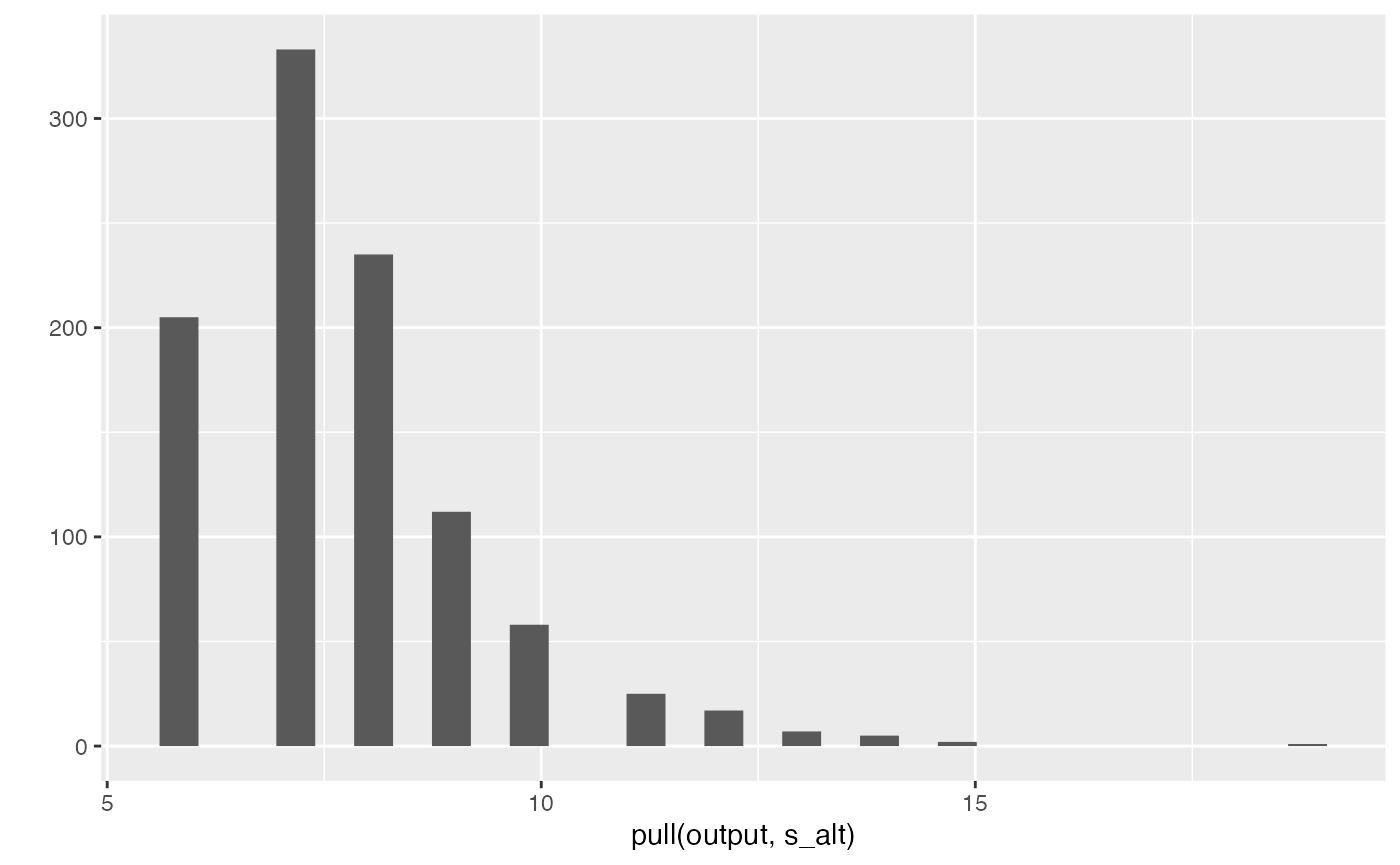
output |> ggplot(aes(max_corr, null_intersection)) +
  geom_point() + geom_smooth(method = "lm")
#> `geom_smooth()` using formula 'y ~ x'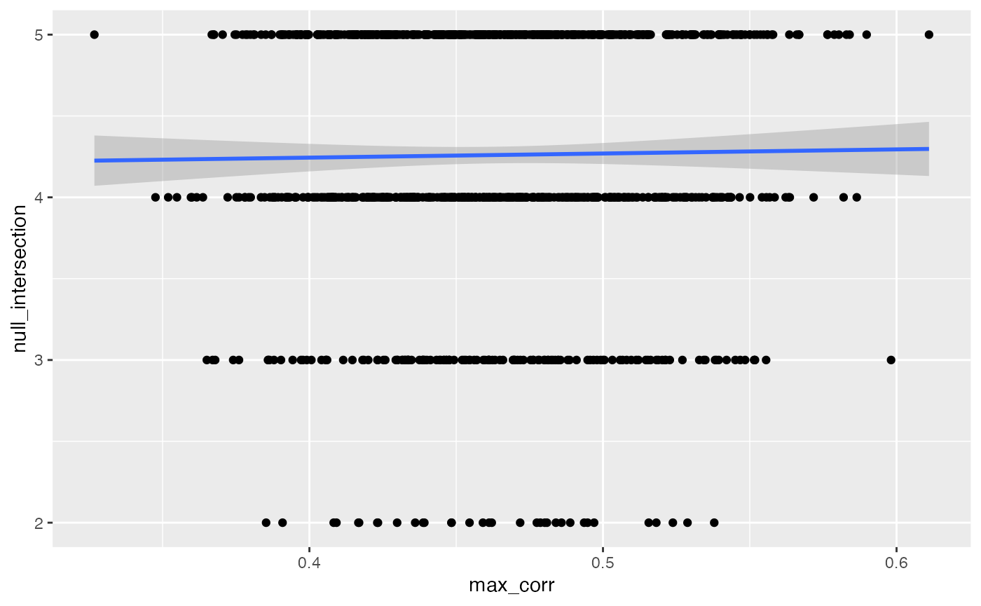
output |> ggplot(aes(min_beta, null_intersection)) +
  geom_point() + geom_smooth(method = "lm")
#> `geom_smooth()` using formula 'y ~ x'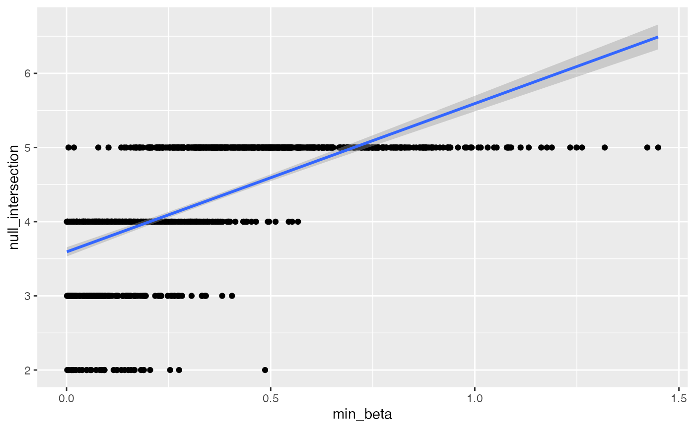
output %>% pull(null_intersection) |> qplot()
#> `stat_bin()` using `bins = 30`. Pick better value with `binwidth`.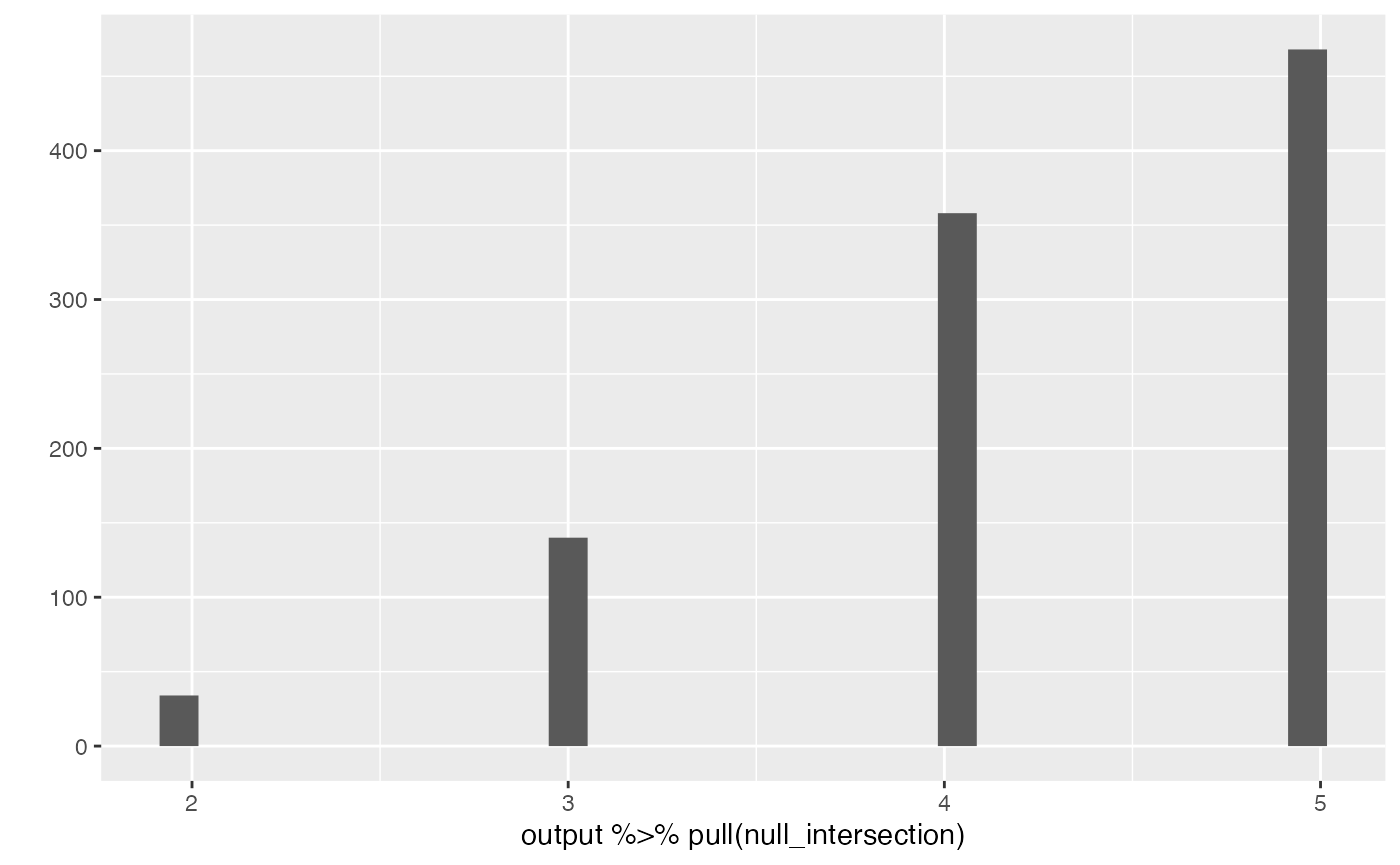
RPtests controls selective error
To the best of my knowledge it is not known whether RPtests is valid for selective inference since it was not designed or proven to do so. This empirical demonstration may be a novel result showing that, at least in the conditions simulated here, the method does control selective errors.